Wildfire risk: standing hazard and right now

This notebook was written by generative AI. It’s meant to show querying across sources/formats, not provide informative analysis. Take the results with a major grain of salt.

Two questions about the same places, stacked on one map:

• Where does it burn? Modelled burn probability and forty years of burn perimeters. These barely change year to year.
• What is happening now? Red Flag Warnings and active fire detections, both of which change by the hour.

Neither alone orders attention very well. A zone with high burn probability is not interesting on a wet day in November; a Red Flag Warning over bare rock is not interesting either. This notebook combines them into a per-zone ranking.

Layer	Source	Velocity	What it tells you
Burn probability	CarbonPlan Open Climate Risk, 1 km	static	How often this pixel burns in a modelled fire regime
Burn history	MTBS perimeters 1984-2024 (Source Cooperative)	static	Whether this landscape actually has a fire regime
Red Flag Warnings	NOAA/NWS active alerts API	minutes	Where fire weather is happening now (wind + low RH + dry fuels)
Active fire detections	NASA FIRMS (MODIS 24h)	hours	Where heat signatures are being detected now

Unit of analysis

The NWS fire weather zone. That is the unit a Red Flag Warning is actually issued for, so nothing has to be downscaled or areally interpolated on the way in.

How it is built

Everything that can be a query is a query. The layers are DuckDB views over remote Parquet, GeoJSON, CSV, and zipped shapefiles (see views.sql), the joins and the geometry work happen in SQL through the spatial extension, and Python is left with the parts it is actually better at: turning raw quantities into weighted scores, drawing, and asserting.

The state is a parameter. One state keeps every layer small enough to work interactively – the whole pipeline below runs in seconds once the HTTP cache is warm.

What the score is and is not

A triage ranking, not a calibrated probability. The weights are a defensible starting point, not a fitted model, and nothing here has been validated against subsequent ignitions. Change WEIGHTS to match what you care about.

Configuration

Everything tunable is here. Nothing below reads a value that is not defined in this cell.

# Wyoming: the most fire zones under a Red Flag Warning in the country at the time of
# writing, with active detections and a real burn history to go with them. Any two-letter
# state works -- see the caveats at the bottom about EPSG:5070 outside CONUS.
STATE = "WY"

# CONUS Albers, for anything that measures an area or a distance
EQUAL_AREA = "EPSG:5070"

# fire just outside a zone boundary still matters
NEARBY_KM = 25.0

# MODIS confidence runs 0-100
MIN_CONFIDENCE = 30

# MTBS also contains prescribed fire, which is not the same signal
WILDFIRE_ONLY = True

# how far past the state line to look for burn perimeters, in degrees
BBOX_PAD_DEG = 0.5

WEIGHTS = {
    "burn_probability": 0.25,  # modelled long-run hazard
    "warning": 0.20,  # under a Red Flag Warning right now
    "detections": 0.20,  # fire already burning inside the zone
    "intensity": 0.10,  # summed FRP, a crude intensity proxy
    "nearby_detections": 0.10,  # fire just outside the boundary
    "burned_share": 0.08,  # share of the zone burned since 1984
    "fire_frequency": 0.07,  # count of distinct historical fires
}
assert abs(sum(WEIGHTS.values()) - 1) < 1e-9, "weights should sum to 1"

from datetime import UTC, datetime

RUN_AT = datetime.now(UTC)
print("Run time (UTC):", RUN_AT.isoformat(timespec="seconds"))
print("State         :", STATE)

Run time (UTC): 2026-09-24T06:20:50+00:00
State         : WY

Configure the import path:

import sys
from pathlib import Path

sys.path.insert(0, str(Path.cwd().parents[1]))

Setup

First, download the burn probabilities.

Pandas

import pandas as pd

pd.set_option("display.max_columns", 100)
pd.set_option("display.max_colwidth", 60)
pd.set_option("display.width", 160)

DuckDB

Docs

import duckdb

%load_ext sql
conn = duckdb.connect()
%sql conn --alias duckdb

/home/runner/work/ptps-wildfire-demo/ptps-wildfire-demo/.venv/lib/python3.14/site-packages/sql/parse.py:339: SyntaxWarning: "\:" is an invalid escape sequence. Such sequences will not work in the future. Did you mean "\\:"? A raw string is also an option.
  Given a query, replaces all occurrences of ':variable' with '\:variable' and
/home/runner/work/ptps-wildfire-demo/ptps-wildfire-demo/.venv/lib/python3.14/site-packages/sql/parse.py:369: SyntaxWarning: "\:" is an invalid escape sequence. Such sequences will not work in the future. Did you mean "\\:"? A raw string is also an option.
  Given a query, replaces all occurrences of 'example'[x:y] with 'example'[x\:y].

Loading configurations from /home/runner/work/ptps-wildfire-demo/ptps-wildfire-demo/pyproject.toml.

Settings changed:

Config	value
autopandas	True
displaycon	False

setup.sql installs the extensions and configures the Source Cooperative credentials; views.sql defines one view per upstream dataset. Binding the views touches every endpoint, so the first run is slow and later ones are served from the cache_httpfs cache.

from helpers import run_script_in_db

run_script_in_db(conn, "setup.sql")
run_script_in_db(conn, "views.sql")

The study area

One state, materialised once. Its bounding box is what keeps every subsequent read small: the burn-probability glob, the FIRMS CSV, and the remote MTBS Parquet are all filtered against it rather than being pulled down whole.

%%sql
CREATE OR REPLACE TABLE study_area AS
SELECT stusps AS state,
    name,
    geom,
    ST_XMin(geom) AS min_lon,
    ST_YMin(geom) AS min_lat,
    ST_XMax(geom) AS max_lon,
    ST_YMax(geom) AS max_lat
FROM state_boundaries
WHERE stusps = '{{STATE}}';

SELECT * EXCLUDE geom FROM study_area;

	state	NAME	min_lon	min_lat	max_lon	max_lat
0	WY	Wyoming	-111.056888	40.996346	-104.052287	45.005904

The fire weather zones are the rows everything else will be attached to. They are stored twice: once in lon/lat for drawing, once in an equal-area projection for measuring.

%%sql
CREATE OR REPLACE TABLE zones AS
SELECT state || 'Z' || zone AS zone_id,
    name AS zone_name,
    state,
    cwa AS forecast_office,
    geom,
    reproject(geom, 'EPSG:4269', '{{EQUAL_AREA}}') AS geom_ea,
    ST_Area(reproject(geom, 'EPSG:4269', '{{EQUAL_AREA}}')) AS zone_area_m2
FROM fire_zones
WHERE state = '{{STATE}}';

SELECT count(*) AS zones,
    round(sum(zone_area_m2) / 1e6) AS total_km2,
    round(median(zone_area_m2) / 1e6) AS median_km2
FROM zones;

	zones	total_km2	median_km2
0	43	252079.0	4953.0

Layer 1 - Burn probability

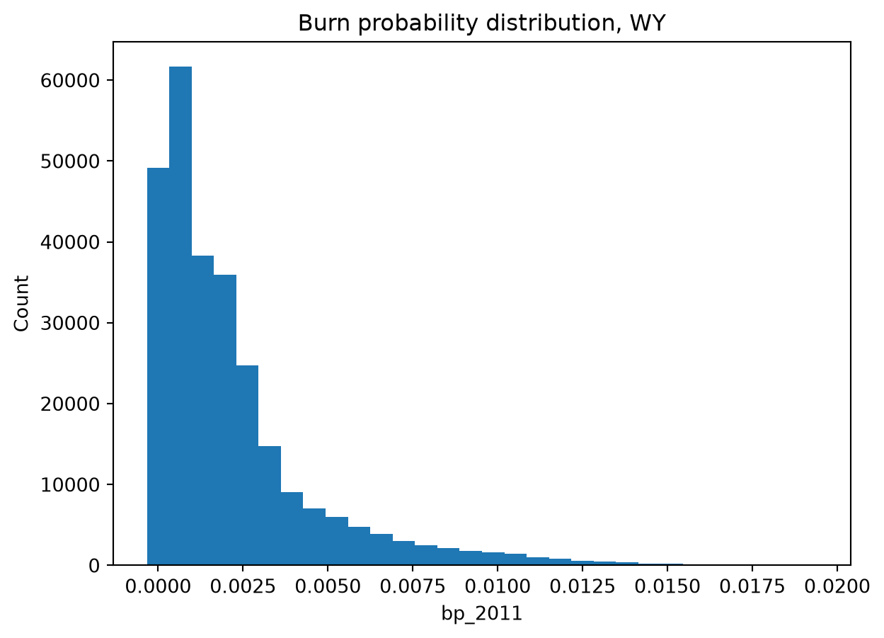
CarbonPlan’s Open Climate Risk burn probability, on a 1 km grid, downloaded by burn_prob.ipynb. bp_2011 is the modelled annual probability that a given pixel burns. The values are small – a 1% annual chance is a lot of fire over a thirty-year mortgage.

%%sql
CREATE OR REPLACE TABLE burn_prob AS
SELECT bp.longitude,
    bp.latitude,
    bp.bp_2011,
    bp.point,
    reproject(ST_Point(bp.longitude, bp.latitude), 'EPSG:4326', '{{EQUAL_AREA}}') AS point_ea
FROM burn_prob_1km AS bp,
    study_area AS s
WHERE bp.bp_2011 IS NOT NULL
    AND NOT isnan(bp.bp_2011)
    -- the raster is CONUS-wide; the bounding box is what makes this cheap
    AND bp.longitude BETWEEN s.min_lon AND s.max_lon
    AND bp.latitude BETWEEN s.min_lat AND s.max_lat;

SELECT count(*) AS cells,
    round(avg(bp_2011), 5) AS mean_bp,
    round(max(bp_2011), 4) AS max_bp
FROM burn_prob;

	cells	mean_bp	max_bp
0	271466	0.00217	0.0191

https://jupysql.readthedocs.io/en/docs/plot.html#histogram

ax = %sqlplot histogram --table burn_prob --column bp_2011 --bins 30
ax.set_title(f"Burn probability distribution, {STATE}")

import folium
from branca.colormap import LinearColormap
from folium.plugins import Fullscreen
import matplotlib.pyplot as plt
import numpy as np
from helpers import add_map_caption, read_geo

state_outline = read_geo(
    conn, "SELECT ST_AsText(geom) AS geom FROM study_area", crs="EPSG:4269"
)
burn_prob_points = conn.execute(
    "SELECT longitude, latitude, bp_2011 FROM burn_prob"
).df()

# interactive: 270k+ points is too many for individual Folium markers, so they're
# rasterised to a transparent image and draped over a pannable basemap at their own
# extent, rather than reinterpreted as a density heatmap
overlay_bounds = (
    burn_prob_points["longitude"].min(),
    burn_prob_points["latitude"].min(),
    burn_prob_points["longitude"].max(),
    burn_prob_points["latitude"].max(),
)
BURN_PROB_CMAP = "RdYlGn_r"

overlay_fig, overlay_ax = plt.subplots(figsize=(8, 8), dpi=150)
overlay_ax.scatter(
    burn_prob_points["longitude"],
    burn_prob_points["latitude"],
    c=burn_prob_points["bp_2011"],
    cmap=BURN_PROB_CMAP,
    s=8,
    linewidths=0,
)
overlay_ax.set_xlim(overlay_bounds[0], overlay_bounds[2])
overlay_ax.set_ylim(overlay_bounds[1], overlay_bounds[3])
overlay_ax.axis("off")
overlay_ax.set_position((0, 0, 1, 1))
overlay_fig.canvas.draw()
overlay_image = np.asarray(overlay_fig.canvas.buffer_rgba())
plt.close(overlay_fig)

m = folium.Map()
m.fit_bounds(
    [[overlay_bounds[1], overlay_bounds[0]], [overlay_bounds[3], overlay_bounds[2]]]
)
folium.raster_layers.ImageOverlay(
    overlay_image,
    bounds=[
        [overlay_bounds[1], overlay_bounds[0]],
        [overlay_bounds[3], overlay_bounds[2]],
    ],
    opacity=0.75,
).add_to(m)
folium.GeoJson(
    state_outline,
    style_function=lambda _: {"color": "black", "weight": 1, "fillOpacity": 0},
).add_to(m)
# scatter() stretches the colormap over the data's range by default, so the legend does too
burn_prob_colors = LinearColormap(
    [plt.get_cmap(BURN_PROB_CMAP)(i / 10) for i in range(11)],
    vmin=burn_prob_points["bp_2011"].min(),
    vmax=burn_prob_points["bp_2011"].max(),
    caption="Annual burn probability",
)
burn_prob_colors.add_to(m)
add_map_caption(m, f"Burn probability, {STATE}", "CarbonPlan Open Climate Risk, 1 km")
Fullscreen().add_to(m)
m

Make this Notebook Trusted to load map: File -> Trust Notebook

Layer 2 - Burn history

MTBS perimeters, 1984-2024, read straight off Source Cooperative. The file covers the whole country and is far too big to download, so the query prunes to nine columns and filters on the perimeter centroid before any geometry is decoded.

DuckDB reads the GeoParquet metadata itself, so geom arrives as a typed GEOMETRY('OGC:CRS84') – no WKB decoding and no guessing at the projection.

%%sql
CREATE OR REPLACE TABLE burn_history AS
SELECT m.event_id,
    m.incident,
    m.incid_type,
    m.acres,
    m.ig_date,
    m.ig_year,
    m.geom,
    reproject(m.geom, 'EPSG:4326', '{{EQUAL_AREA}}') AS geom_ea
FROM mtbs_perimeters AS m,
    study_area AS s
WHERE m.centroid_lon BETWEEN s.min_lon - {{BBOX_PAD_DEG}} AND s.max_lon + {{BBOX_PAD_DEG}}
    AND m.centroid_lat BETWEEN s.min_lat - {{BBOX_PAD_DEG}} AND s.max_lat + {{BBOX_PAD_DEG}}
    AND (
        NOT {{WILDFIRE_ONLY}}
        OR m.incid_type NOT ILIKE '%prescribed%'
    );

SELECT count(*) AS perimeters,
    min(ig_year) AS first_year,
    max(ig_year) AS last_year,
    round(sum(acres) / 1e6, 2) AS million_acres
FROM burn_history;

	perimeters	first_year	last_year	million_acres
0	688	1984	2024	7.45

%%sql
SELECT ig_year, count(*) AS fires, round(sum(acres)) AS acres
FROM burn_history
GROUP BY ig_year
ORDER BY acres DESC
LIMIT 10;

	ig_year	fires	acres
0	1988	49	1738595.0
1	2012	52	689121.0
2	2020	21	627929.0
3	2024	27	579914.0
4	2000	48	539722.0
5	2016	32	336263.0
6	2006	37	333274.0
7	1996	35	313778.0
8	2018	23	278395.0
9	2002	30	219960.0

Layer 3 - Red Flag Warnings

The NWS alerts endpoint returns CAP alerts wrapped in GeoJSON, and most Red Flag Warnings carry geometry: null – they are issued for a zone, not for an ad-hoc polygon. Code that reads the feature’s own geometry silently drops most of the warnings. The red_flag_zones view in views.sql explodes affectedZones and joins each one to its shape from the fire zone shapefile.

The same zone can be covered by more than one alert, so they are collapsed back to one row per zone here.

%%sql
CREATE OR REPLACE TABLE warnings AS
SELECT zone_id,
    count(DISTINCT id) AS n_alerts,
    string_agg(DISTINCT event, ', ') AS events,
    max(severity) AS severity,
    max(expires) AS expires,
    max(headline) AS headline,
    string_agg(DISTINCT senderName, ', ') AS offices
FROM red_flag_zones
WHERE zone_state = '{{STATE}}'
GROUP BY zone_id;

SELECT count(*) AS warned_zones,
    (SELECT count(*) FROM zones) AS zones_in_state,
    min(expires) AS first_expiry,
    max(expires) AS last_expiry
FROM warnings;

	warned_zones	zones_in_state	first_expiry	last_expiry
0	0	43	NaT	NaT

If that came back empty, it is a real answer rather than a failure: Red Flag Warnings are seasonal, and often absent overnight. Every step below still runs – the warning component just scores zero for every zone, and the ranking falls back to standing hazard. Try again during afternoon peak wind, or point STATE somewhere drier.

import folium
from folium.plugins import Fullscreen
from helpers import add_map_caption

zone_outlines = read_geo(
    conn, "SELECT ST_AsText(geom) AS geom FROM zones", crs="EPSG:4269"
)
warned = read_geo(
    conn,
    "SELECT z.zone_id, ST_AsText(z.geom) AS geom "
    "FROM zones AS z JOIN warnings AS w USING (zone_id)",
    crs="EPSG:4269",
)
print(f"{len(warned)} of {len(zone_outlines)} zones warned")

bounds = zone_outlines.total_bounds
m = folium.Map()
m.fit_bounds([[bounds[1], bounds[0]], [bounds[3], bounds[2]]])
folium.GeoJson(
    zone_outlines,
    style_function=lambda _: {"color": "#999999", "weight": 0.5, "fillOpacity": 0},
).add_to(m)
if not warned.empty:
    warning_areas = read_geo(
        conn, "SELECT ST_AsText(geom) AS geom FROM red_flag_warnings", crs="EPSG:4269"
    )
    folium.GeoJson(
        warning_areas,
        style_function=lambda _: {
            "color": "darkred",
            "weight": 1,
            "fillColor": "red",
            "fillOpacity": 0.35,
        },
    ).add_to(m)
add_map_caption(
    m,
    f"Red Flag Warnings, {STATE}",
    f"{RUN_AT:%Y-%m-%d %H:%M} UTC",
    {
        "Red Flag Warning": "background: rgba(255, 0, 0, 0.35); border: 1px solid darkred",
        "fire weather zone": "border: 1px solid #999999",
    },
)
Fullscreen().add_to(m)
m

0 of 43 zones warned

Make this Notebook Trusted to load map: File -> Trust Notebook

Layer 4 - Active fire detections

Each MODIS active fire/thermal hotspot location represents the center of a 1km pixel that is flagged by the algorithm as containing one or more fires within the pixel.

• https://www.earthdata.nasa.gov/data/tools/firms
• https://firms.modaps.eosdis.nasa.gov/active_fire/#firms-txt

A detection is a thermal anomaly, not a confirmed wildfire. Gas flares, industrial heat, and agricultural burning all show up. The bounding box is padded by a degree, because fire on the other side of the state line is still worth counting as nearby.

%%sql
CREATE OR REPLACE TABLE detections AS
SELECT f.latitude,
    f.longitude,
    f.acq_date,
    f.acq_time,
    f.confidence,
    f.frp,
    f.daynight,
    ST_Point(f.longitude, f.latitude) AS point,
    reproject(ST_Point(f.longitude, f.latitude), 'EPSG:4326', '{{EQUAL_AREA}}') AS point_ea
FROM active_fires AS f,
    study_area AS s
WHERE f.longitude BETWEEN s.min_lon - 1 AND s.max_lon + 1
    AND f.latitude BETWEEN s.min_lat - 1 AND s.max_lat + 1
    AND f.confidence >= {{MIN_CONFIDENCE}};

SELECT count(*) AS detections,
    round(sum(frp)) AS total_frp_mw,
    min(acq_date) AS earliest,
    max(acq_date) AS latest
FROM detections;

	detections	total_frp_mw	earliest	latest
0	14	446.0	2026-09-23	2026-09-24

Combining the layers

One query attaches all four layers to each zone. It is written as a function of its input table names so the smoke test at the bottom can run the exact same SQL against fixtures.

Three details worth pointing at:

• Areas and distances are computed in EQUAL_AREA, never in degrees.
• ST_Union_Agg dissolves the burned pieces before measuring them, so a reburn of the same footprint counts as two fires but is only measured once.
• Every count is zero-filled rather than left NULL, so a zone with no fire and no warning is still a row.

def zone_metrics_sql(
    zones="zones",
    detections="detections",
    burn_history="burn_history",
    burn_prob="burn_prob",
    warnings="warnings",
    nearby_m=None,
) -> str:
    """SQL attaching every layer to each zone. Parameterised so fixtures can be swapped in."""
    nearby_m = NEARBY_KM * 1000 if nearby_m is None else nearby_m
    return f"""
WITH inside AS (
    SELECT z.zone_id, count(*) AS n_detections, sum(d.frp) AS frp_sum
    FROM {zones} AS z
    JOIN {detections} AS d ON ST_Contains(z.geom_ea, d.point_ea)
    GROUP BY z.zone_id
),
nearby AS (
    SELECT z.zone_id, count(*) AS n_detections_nearby
    FROM {zones} AS z
    JOIN {detections} AS d ON ST_DWithin(z.geom_ea, d.point_ea, {nearby_m})
    GROUP BY z.zone_id
),
burn_overlaps AS (
    SELECT z.zone_id, h.event_id, h.ig_year,
        ST_Intersection(z.geom_ea, h.geom_ea) AS piece
    FROM {zones} AS z
    JOIN {burn_history} AS h ON ST_Intersects(z.geom_ea, h.geom_ea)
),
history AS (
    SELECT zone_id,
        count(DISTINCT event_id) AS n_hist_fires,
        max(ig_year) AS last_burn_year,
        -- dissolve first, so overlapping reburns aren't double counted
        ST_Area(ST_Union_Agg(piece)) AS burned_m2
    FROM burn_overlaps
    GROUP BY zone_id
),
hazard AS (
    SELECT z.zone_id,
        avg(b.bp_2011) AS mean_burn_prob,
        max(b.bp_2011) AS max_burn_prob,
        count(*) AS n_bp_cells
    FROM {zones} AS z
    JOIN {burn_prob} AS b ON ST_Contains(z.geom_ea, b.point_ea)
    GROUP BY z.zone_id
)
SELECT z.zone_id,
    z.zone_name,
    z.state,
    z.forecast_office,
    z.zone_area_m2,
    w.zone_id IS NOT NULL AS under_warning,
    coalesce(w.n_alerts, 0) AS n_alerts,
    w.events,
    w.severity,
    w.expires,
    w.headline,
    w.offices,
    coalesce(i.n_detections, 0) AS n_detections,
    coalesce(i.frp_sum, 0) AS frp_sum,
    coalesce(n.n_detections_nearby, 0) AS n_detections_nearby,
    coalesce(h.n_hist_fires, 0) AS n_hist_fires,
    h.last_burn_year,
    least(coalesce(h.burned_m2, 0) / z.zone_area_m2, 1.0) AS burned_frac,
    coalesce(hz.mean_burn_prob, 0) AS mean_burn_prob,
    coalesce(hz.max_burn_prob, 0) AS max_burn_prob,
    coalesce(hz.n_bp_cells, 0) AS n_bp_cells,
    z.geom
FROM {zones} AS z
LEFT JOIN {warnings} AS w USING (zone_id)
LEFT JOIN inside AS i USING (zone_id)
LEFT JOIN nearby AS n USING (zone_id)
LEFT JOIN history AS h USING (zone_id)
LEFT JOIN hazard AS hz USING (zone_id)
"""


conn.execute(f"CREATE OR REPLACE TABLE zone_metrics AS {zone_metrics_sql()}")

print(
    f"{conn.execute('SELECT count(*) FROM zone_metrics').fetchone()[0]} zones measured"
)

43 zones measured

%%sql
SELECT zone_id,
    zone_name,
    under_warning,
    n_detections,
    round(frp_sum) AS frp,
    n_detections_nearby,
    n_hist_fires,
    round(burned_frac * 100, 1) AS burned_pct,
    round(mean_burn_prob * 1000, 2) AS burn_prob_per_1k,
    last_burn_year
FROM zone_metrics
ORDER BY under_warning DESC, n_detections DESC, mean_burn_prob DESC
LIMIT 15;

	zone_id	zone_name	under_warning	n_detections	frp	n_detections_nearby	n_hist_fires	burned_pct	burn_prob_per_1k	last_burn_year
0	WYZ285	South Bighorn Mountains	False	2	137.0	3	12	4.0	1.76	2021
1	WYZ274	Sheridan County/Casper BLM	False	1	11.0	1	27	13.1	7.68	2024
2	WYZ284	Bighorn National Forest	False	1	15.0	4	15	5.0	4.54	2021
3	WYZ140	Yellowstone National Park	False	0	0.0	0	53	54.8	6.25	2020
4	WYZ415	North Zone Bridger Teton NF and Grand Teton NP	False	0	0.0	0	35	18.9	5.04	2016
5	WYZ314	Northern Campbell	False	0	0.0	0	34	9.0	4.97	2024
6	WYZ419	North Laramie Range and Adjacent High Plains	False	0	0.0	0	19	14.7	4.84	2018
7	WYZ416	West Wind River Mountains/East Zone Bridger Teton NF	False	0	0.0	0	15	8.1	3.95	2019
8	WYZ424	Sierra Madre Range/Medicine Bow NF	False	0	0.0	0	6	7.1	3.63	2018
9	WYZ300	Casper Mountain	False	0	0.0	0	3	10.2	3.47	2012
10	WYZ286	Absaroka Mountains/North Shoshone NF	False	0	0.0	0	29	14.9	3.36	2019
11	WYZ414	Salt and Wyoming Ranges/West Zone Bridger Teton NF	False	0	0.0	0	16	12.0	3.23	2018
12	WYZ418	Middle North Platte River Basin/Niobrara and Converse Hi...	False	0	0.0	0	35	8.7	3.14	2024
13	WYZ288	East Wind River Mountains/South Shoshone NF	False	0	0.0	0	14	8.1	2.94	2022
14	WYZ429	Southern Laramie Range	False	0	0.0	0	0	0.0	2.75	<NA>

Scoring

Two steps kept deliberately apart: score_components turns raw quantities into comparable 0-1 numbers, and rank_zones applies the weights. So you can inspect the components, reweight without recomputing anything spatial, or drop a component by editing WEIGHTS.

Counts are scaled on a log axis because they are heavily tailed – one zone with forty detections should not flatten every other zone to nothing.

import numpy as np


def scale01(values, log: bool = False) -> pd.Series:
    """Min-max to [0,1]; log1p first for heavy-tailed counts. All-equal -> all zeros."""
    s = pd.to_numeric(pd.Series(values), errors="coerce").fillna(0.0).astype(float)
    if log:
        s = np.log1p(s.clip(lower=0))
    lo, hi = s.min(), s.max()
    if not np.isfinite(lo) or not np.isfinite(hi) or hi <= lo:
        return pd.Series(0.0, index=s.index)
    return (s - lo) / (hi - lo)


def score_components(zones: pd.DataFrame) -> pd.DataFrame:
    """Raw quantities -> comparable 0-1 components."""

    def col(name):
        return (
            zones[name] if name in zones.columns else pd.Series(0.0, index=zones.index)
        )

    return pd.DataFrame(
        {
            "burn_probability": scale01(col("mean_burn_prob")),
            # already 0/1, and scale01 would blow it up to the full range whenever any
            # zone is warned
            "warning": col("under_warning").astype(float),
            "detections": scale01(col("n_detections"), log=True),
            "intensity": scale01(col("frp_sum"), log=True),
            "nearby_detections": scale01(col("n_detections_nearby"), log=True),
            "burned_share": scale01(col("burned_frac")),
            "fire_frequency": scale01(col("n_hist_fires"), log=True),
        },
        index=zones.index,
    )


def rank_zones(zones: pd.DataFrame, weights: dict) -> pd.DataFrame:
    """Weighted composite on a 0-100 scale, with each contribution kept as `c_*`."""
    if zones.empty:
        return zones
    out = zones.copy()
    components = score_components(out)
    for name, weight in weights.items():
        out[f"c_{name}"] = components[name] * weight
    out["score"] = (components * pd.Series(weights)).sum(axis=1) * 100
    out["years_since_burn"] = RUN_AT.year - out["last_burn_year"]
    out = out.sort_values("score", ascending=False).reset_index(drop=True)
    out["rank"] = np.arange(1, len(out) + 1)
    return out

metrics = conn.execute("SELECT * EXCLUDE geom FROM zone_metrics").df()
ranked = rank_zones(metrics, WEIGHTS)

# hand the scores back to DuckDB so the geometry can be joined to them in SQL
conn.register("ranked_df", ranked)
conn.execute("""
CREATE OR REPLACE TABLE zone_ranks AS
SELECT r.*, z.geom
FROM ranked_df AS r
JOIN zones AS z USING (zone_id)
""")

print(
    f"Scored {len(ranked)} zones. Range {ranked['score'].min():.1f}-{ranked['score'].max():.1f}."
)
print("Weights:", ", ".join(f"{k} {v:.0%}" for k, v in WEIGHTS.items()))

Scored 43 zones. Range 1.0-54.7.
Weights: burn_probability 25%, warning 20%, detections 20%, intensity 10%, nearby_detections 10%, burned_share 8%, fire_frequency 7%

The answer

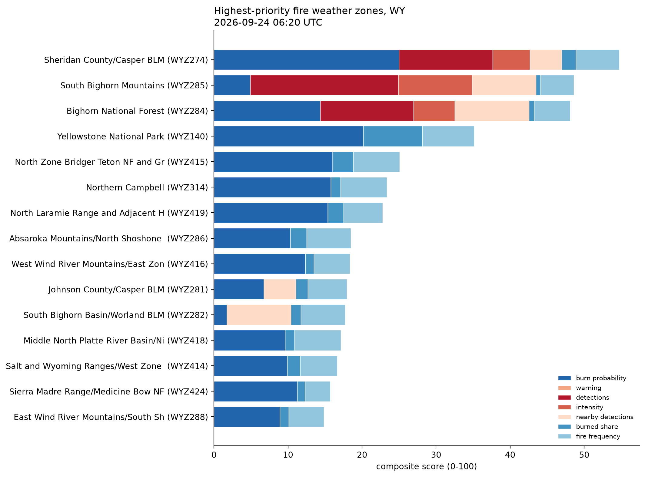
Read the score as a queue order, not a probability.

One deliberate asymmetry worth naming: years_since_burn is reported but not scored. A landscape that burned two years ago is often less dangerous in the short term, because the fuel is gone. Frequency and extent of past fire indicate a fire-prone regime; recency cuts the other way. Folding both into one number would hide that tension, so recency stays a column you read alongside the rank.

%%sql
SELECT rank,
    zone_id,
    zone_name,
    round(score, 1) AS score,
    under_warning,
    n_detections,
    round(frp_sum) AS frp,
    n_detections_nearby,
    round(mean_burn_prob * 1000, 2) AS burn_prob_per_1k,
    round(burned_frac * 100, 1) AS burned_pct,
    n_hist_fires,
    years_since_burn
FROM zone_ranks
ORDER BY rank
LIMIT 20;

	rank	zone_id	zone_name	score	under_warning	n_detections	frp	n_detections_nearby	burn_prob_per_1k	burned_pct	n_hist_fires	years_since_burn
0	1	WYZ274	Sheridan County/Casper BLM	54.7	False	1	11.0	1	7.68	13.1	27	2
1	2	WYZ285	South Bighorn Mountains	48.6	False	2	137.0	3	1.76	4.0	12	5
2	3	WYZ284	Bighorn National Forest	48.1	False	1	15.0	4	4.54	5.0	15	5
3	4	WYZ140	Yellowstone National Park	35.2	False	0	0.0	0	6.25	54.8	53	6
4	5	WYZ415	North Zone Bridger Teton NF and Grand Teton NP	25.1	False	0	0.0	0	5.04	18.9	35	10
5	6	WYZ314	Northern Campbell	23.4	False	0	0.0	0	4.97	9.0	34	2
6	7	WYZ419	North Laramie Range and Adjacent High Plains	22.8	False	0	0.0	0	4.84	14.7	19	8
7	8	WYZ286	Absaroka Mountains/North Shoshone NF	18.5	False	0	0.0	0	3.36	14.9	29	7
8	9	WYZ416	West Wind River Mountains/East Zone Bridger Teton NF	18.4	False	0	0.0	0	3.95	8.1	15	7
9	10	WYZ281	Johnson County/Casper BLM	17.9	False	0	0.0	1	2.31	11.1	19	2
10	11	WYZ282	South Bighorn Basin/Worland BLM	17.7	False	0	0.0	3	0.84	9.4	29	3
11	12	WYZ418	Middle North Platte River Basin/Niobrara and Converse Hi...	17.1	False	0	0.0	0	3.14	8.7	35	2
12	13	WYZ414	Salt and Wyoming Ranges/West Zone Bridger Teton NF	16.6	False	0	0.0	0	3.23	12.0	16	8
13	14	WYZ424	Sierra Madre Range/Medicine Bow NF	15.7	False	0	0.0	0	3.63	7.1	6	8
14	15	WYZ288	East Wind River Mountains/South Shoshone NF	14.8	False	0	0.0	0	2.94	8.1	14	4
15	16	WYZ300	Casper Mountain	14.6	False	0	0.0	0	3.47	10.2	3	14
16	17	WYZ317	Weston County Plains	13.3	False	0	0.0	0	2.44	5.3	19	2
17	18	WYZ426	Snowy Range/Medicine Bow NF	12.4	False	0	0.0	0	1.93	25.6	5	6
18	19	WYZ417	Niobrara/Lower Elevations of Converse/Thunder Basin Nati...	12.2	False	0	0.0	0	2.18	3.4	21	4
19	20	WYZ275	North Bighorn Basin/Worland BLM	12.2	False	0	0.0	3	0.38	1.3	5	8

def describe_hot_zones(ranked: pd.DataFrame, n: int = 5) -> list[str]:
    """One plain-language line per zone that is both warned and actively burning."""
    hot = ranked[(ranked["n_detections"] > 0) & ranked["under_warning"]].head(n)
    return [
        f"{r.zone_name} ({r.zone_id}): {int(r.n_detections)} detections, "
        f"{r.frp_sum:.0f} MW, {r.burned_frac:.0%} of the zone burned since 1984, "
        f"warning expires {r.expires:%b %d %H:%M} UTC"
        for r in hot.itertuples()
    ]


hot = describe_hot_zones(ranked)
print(f"{int((ranked['n_detections'] > 0).sum())} zones have detections inside them.")
print(f"{int(ranked['under_warning'].sum())} zones are under a Red Flag Warning.")
print(f"{len(hot)} are both:\n")
for line in hot:
    print(f"  - {line}")

3 zones have detections inside them.
0 zones are under a Red Flag Warning.
0 are both:

What put each zone where it is

The stacked bars are the weighted contributions, so the segments add up to the score itself. A tall bar made entirely of blue is a standing-hazard zone; one with a lot of red is burning right now.

import matplotlib.pyplot as plt

COMPONENT_COLORS = {
    "burn_probability": "#2166ac",
    "warning": "#f4a582",
    "detections": "#b2182b",
    "intensity": "#d6604d",
    "nearby_detections": "#fddbc7",
    "burned_share": "#4393c3",
    "fire_frequency": "#92c5de",
}


def plot_score_breakdown(ranked, weights, run_at, state, n=15, ax=None):
    if ranked.empty:
        return None
    top = ranked.head(min(n, len(ranked))).iloc[::-1]
    labels = [f"{r.zone_name[:34]} ({r.zone_id})" for r in top.itertuples()]

    if ax is None:
        _, ax = plt.subplots(figsize=(11, 0.42 * len(top) + 2))
    left = np.zeros(len(top))
    for name in weights:
        values = (top[f"c_{name}"] * 100).values
        ax.barh(
            labels,
            values,
            left=left,
            label=name.replace("_", " "),
            color=COMPONENT_COLORS[name],
            edgecolor="white",
            linewidth=0.5,
        )
        left += values

    ax.set_xlabel("composite score (0-100)")
    ax.set_title(
        f"Highest-priority fire weather zones, {state}\n"
        f"{run_at.strftime('%Y-%m-%d %H:%M')} UTC",
        loc="left",
        fontsize=12,
    )
    ax.legend(loc="lower right", fontsize=8, frameon=False)
    ax.spines[["top", "right"]].set_visible(False)
    return ax


plot_score_breakdown(ranked, WEIGHTS, RUN_AT, STATE)
plt.tight_layout()
plt.show()

On the map

Zones shaded by score, with the active detections on top.

import folium
from branca.colormap import linear
from folium.plugins import Fullscreen
from helpers import add_map_caption

ranked_zones = read_geo(
    conn,
    "SELECT zone_id, zone_name, score, under_warning, n_detections, n_hist_fires, "
    "ST_AsText(geom) AS geom FROM zone_ranks",
    crs="EPSG:4269",
)
detection_points = conn.execute(
    "SELECT latitude, longitude, frp, acq_date, confidence FROM detections"
).df()

# interactive: zones coloured by score, with the active detections on top. The same
# colormap fills the zones and draws the legend, so the two can't disagree.
score_colors = linear.YlOrRd_09.scale(
    ranked_zones["score"].min(), ranked_zones["score"].max()
)
score_colors.caption = "Risk score (higher = look first) · ● active fire detection"
bounds = ranked_zones.total_bounds
m = folium.Map()
m.fit_bounds([[bounds[1], bounds[0]], [bounds[3], bounds[2]]])
folium.GeoJson(
    ranked_zones,
    style_function=lambda f: {
        "fillColor": score_colors(f["properties"]["score"]),
        "color": "#787878",
        "weight": 1,
        "fillOpacity": 0.7,
    },
    tooltip=folium.GeoJsonTooltip(
        fields=["zone_name", "score", "n_detections", "n_hist_fires"],
        aliases=["zone", "score", "detections", "historical fires"],
    ),
).add_to(m)
for row in detection_points.itertuples():
    folium.CircleMarker(
        location=[row.latitude, row.longitude],
        radius=3,
        color="#141414",
        fill=True,
        fill_opacity=1,
        tooltip=f"{row.frp:.0f} MW, {row.acq_date}, confidence {row.confidence}",
    ).add_to(m)
score_colors.add_to(m)

add_map_caption(
    m,
    f"Wildfire risk by fire weather zone, {STATE}",
    f"{RUN_AT:%Y-%m-%d %H:%M} UTC",
)
Fullscreen().add_to(m)
m

Make this Notebook Trusted to load map: File -> Trust Notebook

Smoke test

The metrics query is the part most likely to break silently – an empty overlay from a projection mismatch, or a dissolve that stops dissolving, both look like a plausible ranking rather than an error. This builds fixture tables with known answers and runs the same SQL over them.

It needs no network and takes about a second. Run it after editing anything above.

def make_fixtures(conn) -> None:
    """Four zones in a row, with a known number of detections and a known burned area."""
    conn.execute(f"""
    CREATE OR REPLACE TABLE t_zones AS
    SELECT zone_id, zone_name, 'CA' AS state, 'TST' AS forecast_office,
        geom, reproject(geom, 'EPSG:4326', '{EQUAL_AREA}') AS geom_ea,
        ST_Area(reproject(geom, 'EPSG:4326', '{EQUAL_AREA}')) AS zone_area_m2
    FROM (
        SELECT 'TSTZ' || k AS zone_id, 'Test zone ' || k AS zone_name,
            ST_GeomFromText(
                'POLYGON((' || (-122 + k) || ' 36, ' || (-122 + k + 0.6) || ' 36, '
                || (-122 + k + 0.6) || ' 36.6, ' || (-122 + k) || ' 36.6, '
                || (-122 + k) || ' 36))'
            ) AS geom
        FROM range(4) AS t(k)
    );

    -- counts[k] detections inside zone k: 0, 1, 3, 5
    CREATE OR REPLACE TABLE t_detections AS
    SELECT 10.0 * (i + 1) AS frp,
        reproject(ST_Point(-122 + c.k + 0.1 + 0.05 * i, 36.3), 'EPSG:4326', '{EQUAL_AREA}') AS point_ea
    FROM (VALUES (0, 0), (1, 1), (2, 3), (3, 5)) AS c(k, n),
        range(5) AS t(i)
    WHERE i < c.n;

    -- one fire covering a quarter of zone 3, plus a reburn of the same footprint
    CREATE OR REPLACE TABLE t_history AS
    SELECT event_id, ig_year,
        reproject(
            ST_GeomFromText('POLYGON((-119 36, -118.7 36, -118.7 36.3, -119 36.3, -119 36))'),
            'EPSG:4326', '{EQUAL_AREA}'
        ) AS geom_ea
    FROM (VALUES ('A', 1995), ('B', 2015)) AS f(event_id, ig_year);

    -- a constant field, except the eastern end (zone 3) which is hotter
    CREATE OR REPLACE TABLE t_burn_prob AS
    SELECT CASE WHEN lon > -119.4 THEN 0.02 ELSE 0.001 END AS bp_2011,
        reproject(ST_Point(lon, 36.3), 'EPSG:4326', '{EQUAL_AREA}') AS point_ea
    FROM (SELECT -121.9 + 0.1 * i AS lon FROM range(40) AS t(i));

    CREATE OR REPLACE TABLE t_warnings AS
    SELECT 'TSTZ3' AS zone_id, 1 AS n_alerts, 'Red Flag Warning' AS events,
        'Severe' AS severity, TIMESTAMPTZ '2030-01-01 00:00:00Z' AS expires,
        'test' AS headline, 'NWS Test' AS offices;
    """)


def run_smoke_test(conn, weights) -> None:
    make_fixtures(conn)
    sql = zone_metrics_sql(
        zones="t_zones",
        detections="t_detections",
        burn_history="t_history",
        burn_prob="t_burn_prob",
        warnings="t_warnings",
    )
    m = conn.execute(f"{sql} ORDER BY zone_id").df()

    # scale01
    assert scale01([0, 0, 0]).tolist() == [0.0, 0.0, 0.0], (
        "constant input must give zeros"
    )
    assert scale01([0, 5, 10]).tolist() == [0.0, 0.5, 1.0]

    # the detection join
    assert m["n_detections"].tolist() == [0, 1, 3, 5], m["n_detections"].tolist()
    assert m.loc[m.zone_id == "TSTZ0", "frp_sum"].iloc[0] == 0
    assert m.loc[m.zone_id == "TSTZ2", "frp_sum"].iloc[0] == 60.0  # 10 + 20 + 30

    # the burn overlay: two overlapping fires, one footprint
    hit = m[m.zone_id == "TSTZ3"].iloc[0]
    assert hit.n_hist_fires == 2, "distinct fires should be counted separately"
    assert 0.2 < hit.burned_frac < 0.3, f"dissolve failed, got {hit.burned_frac:.3f}"
    assert hit.last_burn_year == 2015
    assert m[m.zone_id == "TSTZ0"].iloc[0].burned_frac == 0

    # warnings and burn probability land on the right zones
    assert m["under_warning"].tolist() == [False, False, False, True]
    assert (
        m.loc[m.zone_id == "TSTZ3", "mean_burn_prob"].iloc[0]
        > (m.loc[m.zone_id == "TSTZ0", "mean_burn_prob"].iloc[0])
    )

    # empty inputs must not raise
    conn.execute("CREATE OR REPLACE TABLE t_none AS SELECT * FROM t_detections LIMIT 0")
    empty = conn.execute(
        zone_metrics_sql(
            zones="t_zones",
            detections="t_none",
            burn_history="t_history",
            burn_prob="t_burn_prob",
            warnings="t_warnings",
        )
    ).df()
    assert (empty["n_detections"] == 0).all()
    assert rank_zones(pd.DataFrame(columns=["zone_id"]), weights).empty

    # ranking: more fire, more history and more hazard should sort higher
    r = rank_zones(m, weights)
    assert r.iloc[0].zone_id == "TSTZ3", r[["zone_id", "score"]].to_dict("records")
    assert r.iloc[-1].zone_id == "TSTZ0"
    assert abs(r["score"].max() - 100) < 1e-6, "top zone maxes every component"

    print(
        f"smoke test passed - {len(r)} fixture zones scored "
        f"{r['score'].min():.1f}-{r['score'].max():.1f}"
    )


run_smoke_test(conn, WEIGHTS)

smoke test passed - 4 fixture zones scored 0.0-100.0

What this does not tell you

• A detection is not a fire. MODIS picks up gas flares, industrial heat, and agricultural burning. High-ranking zones deserve a look at the FIRMS attributes and, in California, the AlertCalifornia camera feeds in the catalog.
• The score is unvalidated. The weights are a starting point, not a fitted model. Nothing here has been checked against subsequent ignitions.
• Burn history cuts both ways. Frequent past fire signals a fire-prone regime; a recent burn usually means depleted fuel. Hence years_since_burn being reported rather than scored.
• MTBS has a size floor and a reporting lag – roughly 1,000 acres in the west, 500 in the east, and it runs a year or more behind. Small and very recent fires are simply absent, so burned_frac is a floor.
• Burn probability is modelled, on a 1 km grid, and averaging it over a zone the size of a county throws away most of what it knows.
• Zones are coarse. A fire weather zone can span a hundred kilometres of very different terrain. Zone-level ranking says “look here”, not “this ridge”.
• Geography. EPSG:5070 is CONUS-appropriate; areas in Alaska, Hawaii, and Puerto Rico will be distorted, and the no-auth FIRMS file covers only CONUS + Hawaii.
• No exposure layer. This ranks hazard, not consequence. Two zones with identical scores can differ enormously in who lives there.
• Nothing is saved. Two of the four layers change by the hour, so re-running this notebook will not reproduce an earlier ranking. Capture anything you need to keep yourself.

Where to take it next, from the same catalog

• Fuel condition – MODIS or Sentinel-2 NDVI as a live dryness proxy; LANDFIRE seasonal fuels for fuel model context. This is the biggest missing driver: the warning tells you the weather, not what is there to burn.
• Exposure and vulnerability – CarbonPlan building-level risk, CDC/ATSDR SVI, EPA EJScreen (archived), and CDC PLACES turn a hazard rank into an impact rank.
• Downwind effects – NOAA HMS smoke polygons plus EPA AirNow move the question from “where will it burn” to “who is breathing it”.
• Response capacity – the OSM extract (hydrants, water lines, roads) and DOE EAGLE-I outage history speak to whether a place can respond.
• Ground truth – WFIGS/NIFC current perimeters, to check whether detections correspond to a recognised, named incident.
• Finer detections – a free FIRMS MAP_KEY upgrades the detection layer from 1 km MODIS to 375 m VIIRS through the Area API.

Most of these slot in as one new view in views.sql, one more CTE in zone_metrics_sql, and one more line in WEIGHTS.